Sentinel Hub Process API
In this example notebook we show how to use Sentinel Hub Process API to download satellite imagery. We describe how to use various parameters and configurations to obtain either processed products or raw band data. For more information about the service please check the official service documentation.
Prerequisites
Credentials
Process API requires Sentinel Hub account. Please check configuration instructions about how to set up your Sentinel Hub credentials.
[1]:
from sentinelhub import SHConfig

config = SHConfig()

if not config.sh_client_id or not config.sh_client_secret:
    print("Warning! To use Process API, please provide the credentials (OAuth client ID and client secret).")
Imports
[2]:
%reload_ext autoreload
%autoreload 2
%matplotlib inline
[3]:
import datetime
import os

import matplotlib.pyplot as plt
import numpy as np

from sentinelhub import (
    CRS,
    BBox,
    DataCollection,
    DownloadRequest,
    MimeType,
    MosaickingOrder,
    SentinelHubDownloadClient,
    SentinelHubRequest,
    bbox_to_dimensions,
)

# The following is not a package. It is a file utils.py which should be in the same folder as this notebook.
from utils import plot_image
Setting area of interest
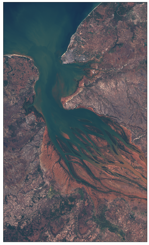
We will download Sentinel-2 imagery of Betsiboka Estuary such as the one shown below (taken by Sentinel-2 on 2017-12-15):
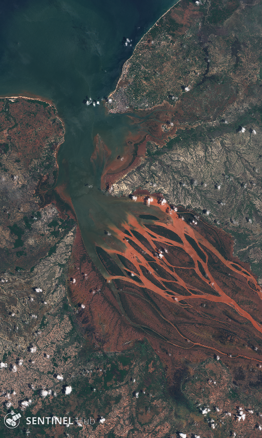
The bounding box in WGS84 coordinate system is [46.16, -16.15, 46.51, -15.58] (longitude and latitude coordinates of lower left and upper right corners). You can get the bbox for a different area at the bboxfinder website.
All requests require bounding box to be given as an instance of sentinelhub.geometry.BBox with corresponding Coordinate Reference System (sentinelhub.constants.CRS). In our case it is in WGS84 and we can use the predefined WGS84 coordinate reference system from sentinelhub.constants.CRS.
[4]:
betsiboka_coords_wgs84 = (46.16, -16.15, 46.51, -15.58)
When the bounding box bounds have been defined, you can initialize the BBox of the area of interest. Using the bbox_to_dimensions utility function, you can provide the desired resolution parameter of the image in meters and obtain the output image shape.
[5]:
resolution = 60
betsiboka_bbox = BBox(bbox=betsiboka_coords_wgs84, crs=CRS.WGS84)
betsiboka_size = bbox_to_dimensions(betsiboka_bbox, resolution=resolution)

print(f"Image shape at {resolution} m resolution: {betsiboka_size} pixels")
Image shape at 60 m resolution: (631, 1047) pixels
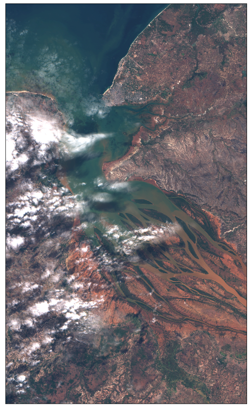
Example 1: True color (PNG) on a specific date
We build the request according to the API Reference, using the SentinelHubRequest class. Each Process API request also needs an evalscript.
The information that we specify in the SentinelHubRequest object is:
an evalscript,
a list of input data collections with time interval,
a format of the response,
a bounding box and it’s size (size or resolution).
The evalscript in the example is used to select the appropriate bands. We return the RGB (B04, B03, B02) Sentinel-2 L1C bands.
The image from Jun 12th 2020 is downloaded. Without any additional parameters in the evalscript, the downloaded data will correspond to reflectance values in UINT8 format (values in 0-255 range).
[6]:
evalscript_true_color = """
    //VERSION=3

    function setup() {
        return {
            input: [{
                bands: ["B02", "B03", "B04"]
            }],
            output: {
                bands: 3
            }
        };
    }

    function evaluatePixel(sample) {
        return [sample.B04, sample.B03, sample.B02];
    }
"""

request_true_color = SentinelHubRequest(
    evalscript=evalscript_true_color,
    input_data=[
        SentinelHubRequest.input_data(
            data_collection=DataCollection.SENTINEL2_L1C,
            time_interval=("2020-06-12", "2020-06-13"),
        )
    ],
    responses=[SentinelHubRequest.output_response("default", MimeType.PNG)],
    bbox=betsiboka_bbox,
    size=betsiboka_size,
    config=config,
)
[7]:
true_color_imgs = request_true_color.get_data()
The method get_data() will always return a list of length 1 with the available image from the requested time interval in the form of numpy arrays.
[8]:
print(f"Returned data is of type = {type(true_color_imgs)} and length {len(true_color_imgs)}.")
print(f"Single element in the list is of type {type(true_color_imgs[-1])} and has shape {true_color_imgs[-1].shape}")
Returned data is of type = <class 'list'> and length 1.
Single element in the list is of type <class 'numpy.ndarray'> and has shape (1047, 631, 3)
[9]:
image = true_color_imgs[0]
print(f"Image type: {image.dtype}")

# plot function
# factor 1/255 to scale between 0-1
# factor 3.5 to increase brightness
plot_image(image, factor=3.5 / 255, clip_range=(0, 1))
Image type: uint8
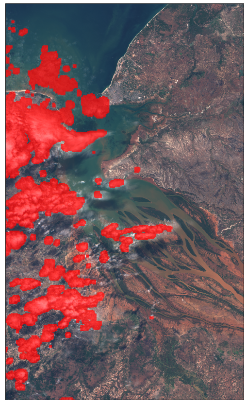
Example 1.1 Adding cloud mask data
It is also possible to obtain cloud masks when requesting Sentinel-2 data by using the cloud mask band (CLM) or the cloud probabilities band (CLP). More info here.
The factor for increasing the image brightness can already be provided in the evalscript.
[10]:
evalscript_clm = """
//VERSION=3
function setup() {
  return {
    input: ["B02", "B03", "B04", "CLM"],
    output: { bands: 3 }
  }
}

function evaluatePixel(sample) {
  if (sample.CLM == 1) {
    return [0.75 + sample.B04, sample.B03, sample.B02]
  }
  return [3.5*sample.B04, 3.5*sample.B03, 3.5*sample.B02];
}
"""

request_true_color = SentinelHubRequest(
    evalscript=evalscript_clm,
    input_data=[
        SentinelHubRequest.input_data(
            data_collection=DataCollection.SENTINEL2_L1C,
            time_interval=("2020-06-12", "2020-06-13"),
        )
    ],
    responses=[SentinelHubRequest.output_response("default", MimeType.PNG)],
    bbox=betsiboka_bbox,
    size=betsiboka_size,
    config=config,
)
[11]:
data_with_cloud_mask = request_true_color.get_data()
[12]:
plot_image(data_with_cloud_mask[0], factor=1 / 255)
Example 2: True color mosaic of least cloudy acquisitions
The SentinelHubRequest automatically creates a mosaic from all available images in the given time interval. By default, the mostRecent mosaicking order is used. More information available here.
In this example we will provide a month long interval, order the images w.r.t. the cloud coverage on the tile level (leastCC parameter), and mosaic them in the specified order.
[13]:
request_true_color = SentinelHubRequest(
    evalscript=evalscript_true_color,
    input_data=[
        SentinelHubRequest.input_data(
            data_collection=DataCollection.SENTINEL2_L1C,
            time_interval=("2020-06-01", "2020-06-30"),
            mosaicking_order=MosaickingOrder.LEAST_CC,
        )
    ],
    responses=[SentinelHubRequest.output_response("default", MimeType.PNG)],
    bbox=betsiboka_bbox,
    size=betsiboka_size,
    config=config,
)
[14]:
plot_image(request_true_color.get_data()[0], factor=3.5 / 255, clip_range=(0, 1))

Example 3: All Sentinel-2’s raw band values
Now let’s define an evalscript which will return all Sentinel-2 spectral bands with raw values.
In this example we are downloading already quite a big chunk of data, so optimization of the request is not out of the question. Downloading raw digital numbers in the INT16 format instead of reflectances in the FLOAT32 format means that much less data is downloaded, which results in a faster download and a smaller usage of SH processing units.
In order to achieve this, we have to set the input units in the evalscript to DN (digital numbers) and the output sampleType argument to INT16. Additionally, we can’t pack all Sentinel-2’s 13 bands into a PNG image, so we have to set the output image type to the TIFF format via MimeType.TIFF in the request.
The digital numbers are in the range from 0-10000, so we have to scale the downloaded data appropriately.
[15]:
evalscript_all_bands = """
    //VERSION=3
    function setup() {
        return {
            input: [{
                bands: ["B01","B02","B03","B04","B05","B06","B07","B08","B8A","B09","B10","B11","B12"],
                units: "DN"
            }],
            output: {
                bands: 13,
                sampleType: "INT16"
            }
        };
    }

    function evaluatePixel(sample) {
        return [sample.B01,
                sample.B02,
                sample.B03,
                sample.B04,
                sample.B05,
                sample.B06,
                sample.B07,
                sample.B08,
                sample.B8A,
                sample.B09,
                sample.B10,
                sample.B11,
                sample.B12];
    }
"""

request_all_bands = SentinelHubRequest(
    evalscript=evalscript_all_bands,
    input_data=[
        SentinelHubRequest.input_data(
            data_collection=DataCollection.SENTINEL2_L1C,
            time_interval=("2020-06-01", "2020-06-30"),
            mosaicking_order=MosaickingOrder.LEAST_CC,
        )
    ],
    responses=[SentinelHubRequest.output_response("default", MimeType.TIFF)],
    bbox=betsiboka_bbox,
    size=betsiboka_size,
    config=config,
)
[16]:
all_bands_response = request_all_bands.get_data()
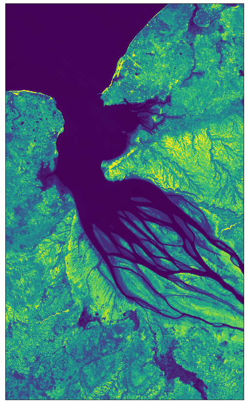
[17]:
# Image showing the SWIR band B12
# Factor 1/1e4 due to the DN band values in the range 0-10000
# Factor 3.5 to increase the brightness
plot_image(all_bands_response[0][:, :, 12], factor=3.5 / 1e4, vmax=1)
[18]:
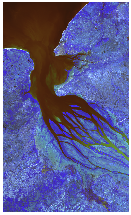
# From raw bands we can also construct a False-Color image
# False color image is (B03, B04, B08)
plot_image(all_bands_response[0][:, :, [2, 3, 7]], factor=3.5 / 1e4, clip_range=(0, 1))
Example 4: Save downloaded data to disk and read it from disk
All downloaded data can be saved to disk and later read from it. Simply specify the location on disk where data should be saved (or loaded from) via the data_folder argument of the request’s constructor. When executing the request’s get_data method, set the argument save_data to True.
This also means that in all the future requests for data, the request will first check the provided location if the data is already there, unless you explicitly demand to redownload the data.
[19]:
request_all_bands = SentinelHubRequest(
    data_folder="test_dir",
    evalscript=evalscript_all_bands,
    input_data=[
        SentinelHubRequest.input_data(
            data_collection=DataCollection.SENTINEL2_L1C,
            time_interval=("2020-06-01", "2020-06-30"),
            mosaicking_order=MosaickingOrder.LEAST_CC,
        )
    ],
    responses=[SentinelHubRequest.output_response("default", MimeType.TIFF)],
    bbox=betsiboka_bbox,
    size=betsiboka_size,
    config=config,
)
[20]:
%%time
all_bands_img = request_all_bands.get_data(save_data=True)
CPU times: user 180 ms, sys: 53.4 ms, total: 234 ms
Wall time: 5.26 s
[21]:
print(
    "The output directory has been created and a tiff file with all 13 bands was saved into the following structure:\n"
)

for folder, _, filenames in os.walk(request_all_bands.data_folder):
    for filename in filenames:
        print(os.path.join(folder, filename))
The output directory has been created and a tiff file with all 13 bands was saved into the following structure:

test_dir/c7cf5a2660a65f3dc8e98e5deddb80d4/request.json
test_dir/c7cf5a2660a65f3dc8e98e5deddb80d4/response.tiff
test_dir/14c9afa9ffb02b037fc61ff8d7d32a81/request.json
test_dir/14c9afa9ffb02b037fc61ff8d7d32a81/response.tiff
[22]:
%%time
# try to re-download the data
all_bands_img_from_disk = request_all_bands.get_data()
CPU times: user 105 ms, sys: 6.32 ms, total: 111 ms
Wall time: 58.7 ms
[23]:
%%time
# force the redownload
all_bands_img_redownload = request_all_bands.get_data(redownload=True)
CPU times: user 173 ms, sys: 47.3 ms, total: 220 ms
Wall time: 6.2 s
Example 4.1: Save downloaded data directly to disk
The get_data method returns a list of numpy arrays and can save the downloaded data to disk, as we have seen in the previous example. Sometimes it is convenient to just save the data directly to disk. You can do that by using save_data method instead.
[24]:
%%time
request_all_bands.save_data()
CPU times: user 310 µs, sys: 109 µs, total: 419 µs
Wall time: 382 µs
[25]:
print(
    "The output directory has been created and a tiff file with all 13 bands was saved into the following structure:\n"
)

for folder, _, filenames in os.walk(request_all_bands.data_folder):
    for filename in filenames:
        print(os.path.join(folder, filename))
The output directory has been created and a tiff file with all 13 bands was saved into the following structure:

test_dir/c7cf5a2660a65f3dc8e98e5deddb80d4/request.json
test_dir/c7cf5a2660a65f3dc8e98e5deddb80d4/response.tiff
test_dir/14c9afa9ffb02b037fc61ff8d7d32a81/request.json
test_dir/14c9afa9ffb02b037fc61ff8d7d32a81/response.tiff
Example 5: Other Data Collections
The sentinelhub-py package supports various data collections. The example below is shown for one of them, but the process is the same for all of them.
Note:
For more examples and information check the tutorial about data collections and Sentinel Hub documentation about data collections.
[26]:
print("Supported DataCollections:\n")
for collection in DataCollection.get_available_collections():
    print(collection)
Supported DataCollections:

DataCollection.SENTINEL2_L1C
DataCollection.SENTINEL2_L2A
DataCollection.SENTINEL1
DataCollection.SENTINEL1_IW
DataCollection.SENTINEL1_IW_ASC
DataCollection.SENTINEL1_IW_DES
DataCollection.SENTINEL1_EW
DataCollection.SENTINEL1_EW_ASC
DataCollection.SENTINEL1_EW_DES
DataCollection.SENTINEL1_EW_SH
DataCollection.SENTINEL1_EW_SH_ASC
DataCollection.SENTINEL1_EW_SH_DES
DataCollection.DEM
DataCollection.DEM_MAPZEN
DataCollection.DEM_COPERNICUS_30
DataCollection.DEM_COPERNICUS_90
DataCollection.MODIS
DataCollection.LANDSAT_MSS_L1
DataCollection.LANDSAT_TM_L1
DataCollection.LANDSAT_TM_L2
DataCollection.LANDSAT_ETM_L1
DataCollection.LANDSAT_ETM_L2
DataCollection.LANDSAT_OT_L1
DataCollection.LANDSAT_OT_L2
DataCollection.SENTINEL5P
DataCollection.SENTINEL3_OLCI
DataCollection.SENTINEL3_SLSTR
For this example let’s download the digital elevation model data (DEM). The process is similar as before, we just provide the evalscript and create the request. More data on the DEM data collection is available here. DEM values are in meters and can be negative for areas which lie below sea level, so it is recommended to set the output format in your evalscript to FLOAT32.
[27]:
evalscript_dem = """
//VERSION=3
function setup() {
  return {
    input: ["DEM"],
    output:{
      id: "default",
      bands: 1,
      sampleType: SampleType.FLOAT32
    }
  }
}

function evaluatePixel(sample) {
  return [sample.DEM]
}
"""
[28]:
dem_request = SentinelHubRequest(
    evalscript=evalscript_dem,
    input_data=[
        SentinelHubRequest.input_data(
            data_collection=DataCollection.DEM,
            time_interval=("2020-06-12", "2020-06-13"),
        )
    ],
    responses=[SentinelHubRequest.output_response("default", MimeType.TIFF)],
    bbox=betsiboka_bbox,
    size=betsiboka_size,
    config=config,
)
[29]:
dem_data = dem_request.get_data()
[30]:
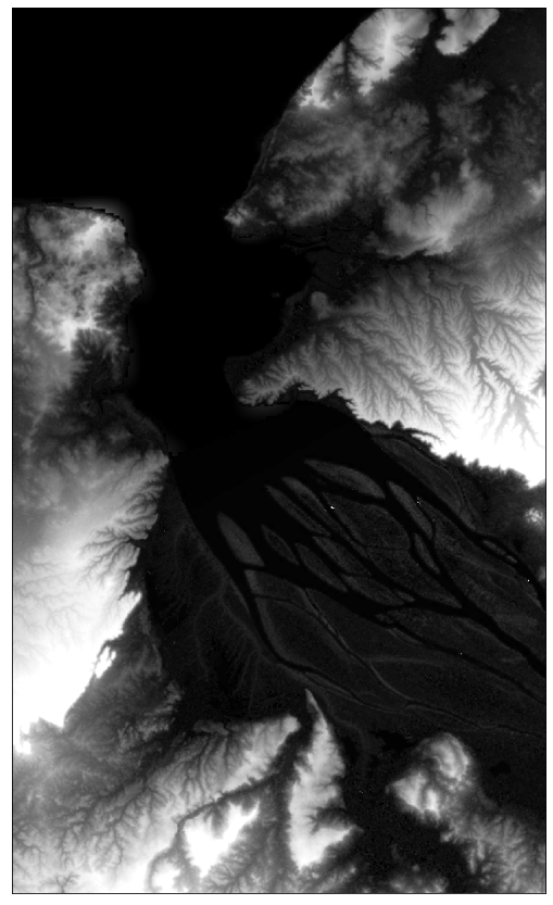
# Plot DEM map
# vmin = 0; cutoff at sea level (0 m)
# vmax = 120; cutoff at high values (120 m)
plot_image(dem_data[0], factor=1.0, cmap=plt.cm.Greys_r, vmin=0, vmax=120)
Example 6 : Multi-response request type
Process API enables downloading multiple files in one response, packed together in a TAR archive.
We will get the same image as before, download in the form of digital numbers (DN) as a UINT16 TIFF file. Along with the image we will download the inputMetadata which contains the normalization factor value in a JSON format.
After the download we will be able to convert the INT16 digital numbers to get the FLOAT32 reflectances.
[31]:
evalscript = """
    //VERSION=3

    function setup() {
        return {
            input: [{
                bands: ["B02", "B03", "B04"],
                units: "DN"
            }],
            output: {
                bands: 3,
                sampleType: "INT16"
            }
        };
    }

    function updateOutputMetadata(scenes, inputMetadata, outputMetadata) {
        outputMetadata.userData = { "norm_factor":  inputMetadata.normalizationFactor }
    }

    function evaluatePixel(sample) {
        return [sample.B04, sample.B03, sample.B02];
    }
"""

request_multitype = SentinelHubRequest(
    evalscript=evalscript,
    input_data=[
        SentinelHubRequest.input_data(
            data_collection=DataCollection.SENTINEL2_L1C,
            time_interval=("2020-06-01", "2020-06-30"),
            mosaicking_order=MosaickingOrder.LEAST_CC,
        )
    ],
    responses=[
        SentinelHubRequest.output_response("default", MimeType.TIFF),
        SentinelHubRequest.output_response("userdata", MimeType.JSON),
    ],
    bbox=betsiboka_bbox,
    size=betsiboka_size,
    config=config,
)
[32]:
# print out information
multi_data = request_multitype.get_data()[0]
multi_data.keys()
[32]:
dict_keys(['default.tif', 'userdata.json'])
[33]:
# normalize image
img = multi_data["default.tif"]
norm_factor = multi_data["userdata.json"]["norm_factor"]

img_float32 = img * norm_factor
[34]:
plot_image(img_float32, factor=3.5, clip_range=(0, 1))
Example 7 : Raw dictionary request
All requests so far were built with some helper functions. We can also construct a raw dictionary as defined in the API Reference, without these helper functions, so we have full control over building the request body.
[35]:
request_raw_dict = {
    "input": {
        "bounds": {"properties": {"crs": betsiboka_bbox.crs.opengis_string}, "bbox": list(betsiboka_bbox)},
        "data": [
            {
                "type": "S2L1C",
                "dataFilter": {
                    "timeRange": {"from": "2020-06-01T00:00:00Z", "to": "2020-06-30T00:00:00Z"},
                    "mosaickingOrder": "leastCC",
                },
            }
        ],
    },
    "output": {
        "width": betsiboka_size[0],
        "height": betsiboka_size[1],
        "responses": [{"identifier": "default", "format": {"type": MimeType.TIFF.get_string()}}],
    },
    "evalscript": evalscript_true_color,
}
[36]:
# create request
download_request = DownloadRequest(
    request_type="POST",
    url="https://services.sentinel-hub.com/api/v1/process",
    post_values=request_raw_dict,
    data_type=MimeType.TIFF,
    headers={"content-type": "application/json"},
    use_session=True,
)

# execute request
client = SentinelHubDownloadClient(config=config)
img = client.download(download_request)
[37]:
plot_image(img, factor=3.5 / 255, clip_range=(0, 1))

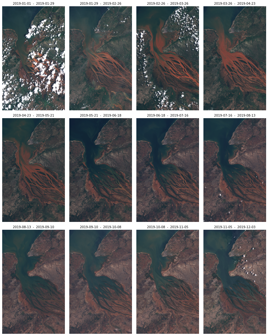
Example 8 : Multiple timestamps data
It is possible to construct some logic in order to return data for multiple timestamps. By defining the time_interval parameter and some logic of splitting it, it is possible to create an SH reques per each “time slot” and then download the data from all the requests with the SentinelHubDownloadClient in sentinelhub-py. In this example we will create least cloudy monthly images for the year 2019.
However, this is already a functionality built on top of this SH API package. We have extended the support for such usage in our package eo-learn. We recommend to use eo-learn for more complex cases where you need multiple timestamps or high-resolution data for larger areas.
[38]:
start = datetime.datetime(2019, 1, 1)
end = datetime.datetime(2019, 12, 31)
n_chunks = 13
tdelta = (end - start) / n_chunks
edges = [(start + i * tdelta).date().isoformat() for i in range(n_chunks)]
slots = [(edges[i], edges[i + 1]) for i in range(len(edges) - 1)]

print("Monthly time windows:\n")
for slot in slots:
    print(slot)
Monthly time windows:

('2019-01-01', '2019-01-29')
('2019-01-29', '2019-02-26')
('2019-02-26', '2019-03-26')
('2019-03-26', '2019-04-23')
('2019-04-23', '2019-05-21')
('2019-05-21', '2019-06-18')
('2019-06-18', '2019-07-16')
('2019-07-16', '2019-08-13')
('2019-08-13', '2019-09-10')
('2019-09-10', '2019-10-08')
('2019-10-08', '2019-11-05')
('2019-11-05', '2019-12-03')
[39]:
def get_true_color_request(time_interval):
    return SentinelHubRequest(
        evalscript=evalscript_true_color,
        input_data=[
            SentinelHubRequest.input_data(
                data_collection=DataCollection.SENTINEL2_L1C,
                time_interval=time_interval,
                mosaicking_order=MosaickingOrder.LEAST_CC,
            )
        ],
        responses=[SentinelHubRequest.output_response("default", MimeType.PNG)],
        bbox=betsiboka_bbox,
        size=betsiboka_size,
        config=config,
    )
[40]:
# create a list of requests
list_of_requests = [get_true_color_request(slot) for slot in slots]
list_of_requests = [request.download_list[0] for request in list_of_requests]

# download data with multiple threads
data = SentinelHubDownloadClient(config=config).download(list_of_requests, max_threads=5)
[41]:
# some stuff for pretty plots
ncols = 4
nrows = 3
aspect_ratio = betsiboka_size[0] / betsiboka_size[1]
subplot_kw = {"xticks": [], "yticks": [], "frame_on": False}

fig, axs = plt.subplots(ncols=ncols, nrows=nrows, figsize=(5 * ncols * aspect_ratio, 5 * nrows), subplot_kw=subplot_kw)

for idx, image in enumerate(data):
    ax = axs[idx // ncols][idx % ncols]
    ax.imshow(np.clip(image * 2.5 / 255, 0, 1))
    ax.set_title(f"{slots[idx][0]}  -  {slots[idx][1]}", fontsize=10)

plt.tight_layout()