Large area utilities
Many times we would like to run algorithms for large geographical areas. However due to large amount of data we probably won’t have enough working memory to do that all at once. So we need to split the area into smaller parts and properly manage them. To make this easier sentinelhub package implements utilities for splitting areas into smaller bounding boxes.
Prerequisites
Imports
[4]:
%matplotlib inline
# ruff: noqa: I001
import itertools
import tempfile
from pathlib import Path

import numpy as np
from shapely.geometry import MultiLineString, MultiPolygon, Polygon, box, shape

from sentinelhub import (
    CRS,
    BBox,
    BBoxSplitter,
    CustomGridSplitter,
    DataCollection,
    MimeType,
    MosaickingOrder,
    OsmSplitter,
    SentinelHubDownloadClient,
    SentinelHubRequest,
    TileSplitter,
    UtmGridSplitter,
    UtmZoneSplitter,
    read_data,
)
The following packages are not included or required for sentinelhub package however they are used in this example notebook. In case you would like to reproduce some visualizations you will have to install them separately.
[5]:
import geopandas as gpd
import matplotlib.pyplot as plt
import rioxarray  # noqa: F401 # Its necesary for xarray.open_mfdataset() with engine `rasterio`
import xarray as xr  # It may need Dask library https://docs.dask.org/en/stable/install.html
from matplotlib.patches import Polygon as PltPolygon
from mpl_toolkits.basemap import Basemap  # Available here: https://github.com/matplotlib/basemap
Collecting data
To start we need a geometry of the area of interest. The sentinelhub package uses the shapely package to work with geometries. Therefore any geometry inputs need to be an instance of shapely.geometry.multipolygon.MultiPolygon or shapely.geometry.polygon.Polygon.
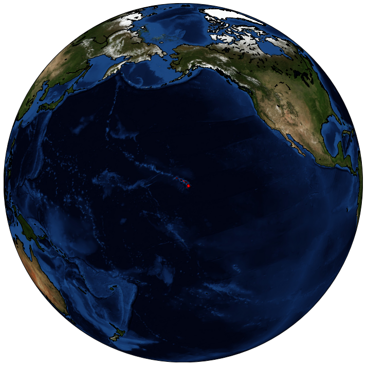
In these examples we will use a geometry of Hawaii islands.
[6]:
# ruff: noqa: C901

INPUT_FILE = "./data/Hawaii.json"

geo_json = read_data(INPUT_FILE)
hawaii_area = shape(geo_json["features"][0]["geometry"])

type(hawaii_area)
[6]:
shapely.geometry.multipolygon.MultiPolygon
Let’s check how the area looks on the world map.
[7]:
def show_area(area_shape):
    fig = plt.figure(figsize=(10, 10))
    ax = fig.add_subplot(111)

    minx, miny, maxx, maxy = area_shape.bounds
    lng, lat = (minx + maxx) / 2, (miny + maxy) / 2

    m = Basemap(projection="ortho", lat_0=lat, lon_0=lng, resolution="l")
    m.drawcoastlines()
    m.bluemarble()

    if isinstance(area_shape, Polygon):
        polygon_iter = [area_shape]
    elif isinstance(area_shape, MultiPolygon):
        polygon_iter = area_shape.geoms
    else:
        raise ValueError(f"Geometry of type {type(area_shape)} is not supported")

    for polygon in polygon_iter:
        x, y = np.array(polygon.boundary.coords)[0]
        m_poly = []
        for x, y in np.array(polygon.boundary.coords):
            m_poly.append(m(x, y))
        ax.add_patch(PltPolygon(np.array(m_poly), closed=True, facecolor="red", edgecolor="red"))

    plt.tight_layout()
    plt.show()


show_area(hawaii_area)
Clipping input data to the valid range for imshow with RGB data ([0..1] for floats or [0..255] for integers).
Area Splitting
We would like to split the area into smaller bounding boxes which could them be used for obtaining data by calling WMS/WCS requests. The package implements 3 different ways of splitting the area.
Splitting the bounding box
The most straight forward approach is to calculate the area bounding box and split it into smaller parts of equal size.
As an input we need to provide a list of geometries, their CRS, and int or tuple specifying to how many parts bounding box will be split.
[8]:
bbox_splitter = BBoxSplitter(
    [hawaii_area], CRS.WGS84, (5, 4)
)  # bounding box will be split into grid of 5x4 bounding boxes

print("Area bounding box: {}\n".format(bbox_splitter.get_area_bbox().__repr__()))

bbox_list = bbox_splitter.get_bbox_list()
info_list = bbox_splitter.get_info_list()

print(
    "Each bounding box also has some info how it was created.\nExample:\nbbox: {}\ninfo: {}\n".format(
        bbox_list[0].__repr__(), info_list[0]
    )
)
Area bounding box: BBox(((-159.764448, 18.948267), (-154.807817, 22.228955)), crs=CRS('4326'))

Each bounding box also has some info how it was created.
Example:
bbox: BBox(((-159.764448, 21.408783), (-158.77312179999998, 22.228955)), crs=CRS('4326'))
info: {'parent_bbox': BBox(((-159.764448, 18.948267), (-154.807817, 22.228955)), crs=CRS('4326')), 'index_x': 0, 'index_y': 3}
Besides the list of bounding boxes it is also possible to get a list of geometries (i.e. intersection of each bounding box with entire area of interest).
[9]:
geometry_list = bbox_splitter.get_geometry_list()

geometry_list[0]
[9]:

In order to visualize the splits let’s use the following function
[10]:
def show_splitter(splitter, alpha=0.2, area_buffer=0.2, show_legend=False):
    area_bbox = splitter.get_area_bbox()
    minx, miny, maxx, maxy = area_bbox
    lng, lat = area_bbox.middle
    w, h = maxx - minx, maxy - miny
    minx = minx - area_buffer * w
    miny = miny - area_buffer * h
    maxx = maxx + area_buffer * w
    maxy = maxy + area_buffer * h

    fig = plt.figure(figsize=(10, 10))
    ax = fig.add_subplot(111)

    base_map = Basemap(
        projection="mill",
        lat_0=lat,
        lon_0=lng,
        llcrnrlon=minx,
        llcrnrlat=miny,
        urcrnrlon=maxx,
        urcrnrlat=maxy,
        resolution="l",
        epsg=4326,
    )
    base_map.drawcoastlines(color=(0, 0, 0, 0))

    area_shape = splitter.get_area_shape()

    if isinstance(area_shape, Polygon):
        polygon_iter = [area_shape]
    elif isinstance(area_shape, MultiPolygon):
        polygon_iter = area_shape.geoms
    else:
        raise ValueError(f"Geometry of type {type(area_shape)} is not supported")

    for polygon in polygon_iter:
        if isinstance(polygon.boundary, MultiLineString):
            for linestring in polygon.boundary:
                ax.add_patch(PltPolygon(np.array(linestring), closed=True, facecolor=(0, 0, 0, 0), edgecolor="red"))
        else:
            ax.add_patch(
                PltPolygon(np.array(polygon.boundary.coords), closed=True, facecolor=(0, 0, 0, 0), edgecolor="red")
            )

    bbox_list = splitter.get_bbox_list()
    info_list = splitter.get_info_list()

    cm = plt.get_cmap("jet", len(bbox_list))
    legend_shapes = []
    for i, bbox in enumerate(bbox_list):
        wgs84_bbox = bbox.transform(CRS.WGS84).get_polygon()

        tile_color = tuple(list(cm(i))[:3] + [alpha])
        ax.add_patch(PltPolygon(np.array(wgs84_bbox), closed=True, facecolor=tile_color, edgecolor="green"))

        if show_legend:
            legend_shapes.append(plt.Rectangle((0, 0), 1, 1, fc=cm(i)))

    if show_legend:
        legend_names = []
        for info in info_list:
            legend_name = "{},{}".format(info["index_x"], info["index_y"])

            for prop in ["grid_index", "tile"]:
                if prop in info:
                    legend_name = "{},{}".format(info[prop], legend_name)

            legend_names.append(legend_name)

        plt.legend(legend_shapes, legend_names)
    plt.tight_layout()
    plt.show()
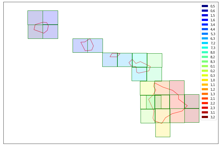
[11]:
show_splitter(bbox_splitter, show_legend=True)
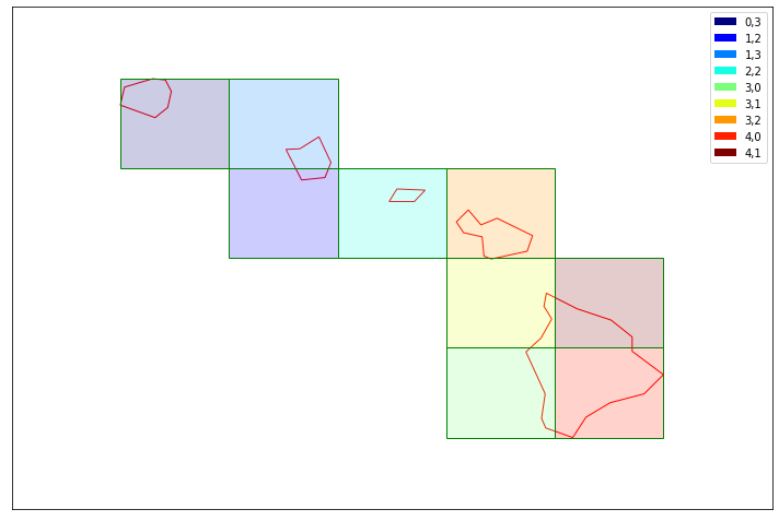
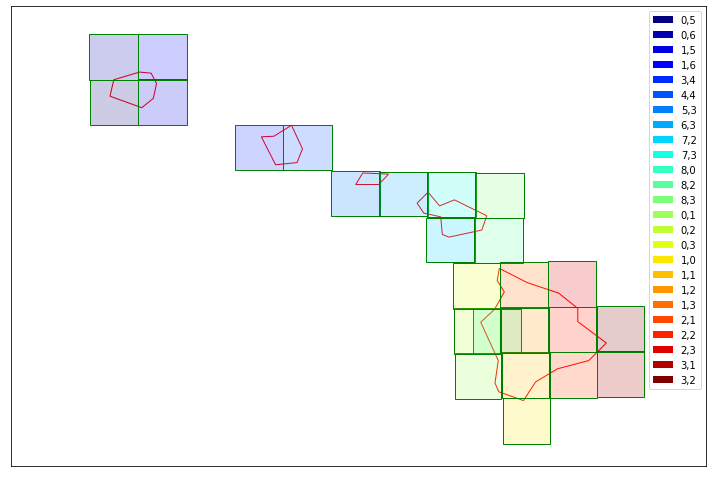
Splitter automatically removed the bounding boxes that did not intersect with the geometry of Hawaii Islands. However the majority of the area inside bounding boxes is still outside our geometry. Therefore each splitter has also an optional parameter reduce_bbox_sizes.
[12]:
bbox_splitter_reduced = BBoxSplitter([hawaii_area], CRS.WGS84, (5, 4), reduce_bbox_sizes=True)

show_splitter(bbox_splitter_reduced, show_legend=True)
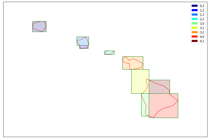
By specifying finer splitting we could even further reduce the total area of bounding boxes.
Splitting in OSM grid
Sometimes it is better to have a splitting grid independent from the given geometries. That way if the geometries at some point slightly change the grid will stay the same.
The following splitter implements Open Street Map’s grid.
[13]:
osm_splitter = OsmSplitter([hawaii_area], CRS.WGS84, zoom_level=10)

print(repr(osm_splitter.get_bbox_list()[0]))
print(osm_splitter.get_info_list()[0])
BBox(((-159.96093749999997, 21.616579336740603), (-159.609375, 21.943045533438177)), crs=CRS('4326'))
{'zoom_level': 10, 'index_x': 57, 'index_y': 448}
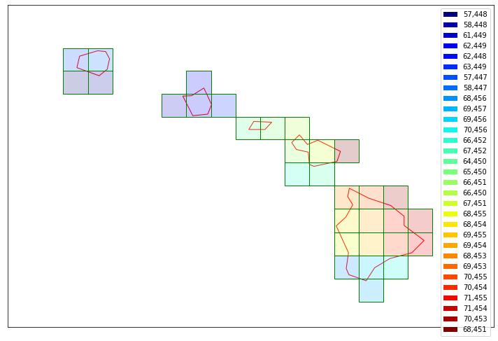
[14]:
show_splitter(osm_splitter, show_legend=True)
Splitting in satellite’s tile grid
If we would like to work on a level of satellite tiles and split them we can use the TileSplitter. It works in combination with Sentinel Hub WFS service therefore an instance ID is required, as described in instruction. We also need to specify time_interval and data_collection.
[15]:
from sentinelhub import SHConfig

config = SHConfig()

if config.instance_id == "":
    print("Warning! To use WFS functionality, please configure the `instance_id`.")
[16]:
tile_splitter = TileSplitter(
    [hawaii_area], CRS.WGS84, ("2017-10-01", "2017-11-01"), data_collection=DataCollection.SENTINEL2_L1C, config=config
)

tile_bbox_list = tile_splitter.get_bbox_list()

print(len(tile_bbox_list))
print(tile_bbox_list[0].__repr__())
print(tile_splitter.get_info_list()[0])
16
BBox(((699960.0, 2290200.0), (809760.0, 2400000.0)), crs=CRS('32604'))
{'parent_bbox': BBox(((699960.0, 2290200.0), (809760.0, 2400000.0)), crs=CRS('32604')), 'index_x': 0, 'index_y': 0, 'ids': ['S2B_MSIL1C_20171028T210909_N0206_R057_T04QGJ_20171028T223108', 'S2A_MSIL1C_20171013T210921_N0205_R057_T04QGJ_20171013T210922', 'S2B_MSIL1C_20171008T210909_N0205_R057_T04QGJ_20171008T210909'], 'timestamps': [datetime.datetime(2017, 10, 28, 21, 9, 10, tzinfo=tzutc()), datetime.datetime(2017, 10, 13, 21, 9, 22, tzinfo=tzutc()), datetime.datetime(2017, 10, 8, 21, 9, 9, tzinfo=tzutc())]}
TileSplitter by default returns bounding boxes in the satellite tile CRS. In order to transform them we can use BBox.transform(target_crs) method or by specifying crs parameter in get_bbox_list method.
Note: This will only transform bounding box vertices and therefore the new bounding box will not be completely aligned with the original one.
[17]:
tile_splitter.get_bbox_list(crs=CRS.WGS84)[0]
[17]:
BBox(((-157.08006491221116, 20.700623752178174), (-156.0067983462315, 21.676398866470976)), crs=CRS('4326'))
[18]:
show_splitter(tile_splitter)
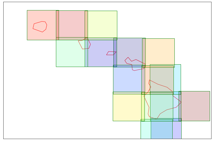
Obtained Sentinel-2 tiles intersect each other. Therefore this splitter is only useful if we are analyzing data on level of original satellite tiles.
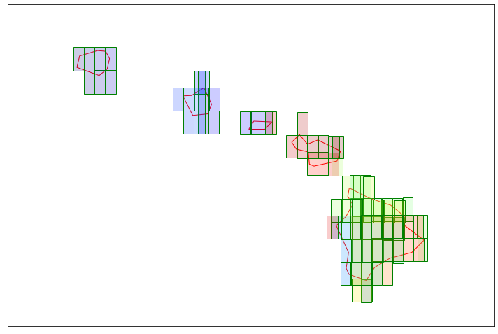
We can also specify to further split the satellite tiles.
[19]:
finer_tile_splitter = TileSplitter(
    [hawaii_area],
    CRS.WGS84,
    ("2017-10-01", "2018-03-01"),
    tile_split_shape=(7, 3),
    data_collection=DataCollection.SENTINEL2_L1C,
    config=config,
)

show_splitter(finer_tile_splitter, show_legend=False)
Splitting in custom grid
In case none of the above splitters suffices there is also a CustomGridSplitter. All we need is a list of bounding boxes, which define a new way of splitting the area.
The following example is just a split into bounding boxes with integer value latitude and longitude:
[20]:
bbox_grid = [BBox((x, y, x + 1, y + 1), CRS.WGS84) for x, y in itertools.product(range(-159, -155), range(18, 23))]

bbox_grid
[20]:
[BBox(((-159.0, 18.0), (-158.0, 19.0)), crs=CRS('4326')),
 BBox(((-159.0, 19.0), (-158.0, 20.0)), crs=CRS('4326')),
 BBox(((-159.0, 20.0), (-158.0, 21.0)), crs=CRS('4326')),
 BBox(((-159.0, 21.0), (-158.0, 22.0)), crs=CRS('4326')),
 BBox(((-159.0, 22.0), (-158.0, 23.0)), crs=CRS('4326')),
 BBox(((-158.0, 18.0), (-157.0, 19.0)), crs=CRS('4326')),
 BBox(((-158.0, 19.0), (-157.0, 20.0)), crs=CRS('4326')),
 BBox(((-158.0, 20.0), (-157.0, 21.0)), crs=CRS('4326')),
 BBox(((-158.0, 21.0), (-157.0, 22.0)), crs=CRS('4326')),
 BBox(((-158.0, 22.0), (-157.0, 23.0)), crs=CRS('4326')),
 BBox(((-157.0, 18.0), (-156.0, 19.0)), crs=CRS('4326')),
 BBox(((-157.0, 19.0), (-156.0, 20.0)), crs=CRS('4326')),
 BBox(((-157.0, 20.0), (-156.0, 21.0)), crs=CRS('4326')),
 BBox(((-157.0, 21.0), (-156.0, 22.0)), crs=CRS('4326')),
 BBox(((-157.0, 22.0), (-156.0, 23.0)), crs=CRS('4326')),
 BBox(((-156.0, 18.0), (-155.0, 19.0)), crs=CRS('4326')),
 BBox(((-156.0, 19.0), (-155.0, 20.0)), crs=CRS('4326')),
 BBox(((-156.0, 20.0), (-155.0, 21.0)), crs=CRS('4326')),
 BBox(((-156.0, 21.0), (-155.0, 22.0)), crs=CRS('4326')),
 BBox(((-156.0, 22.0), (-155.0, 23.0)), crs=CRS('4326'))]
[21]:
custom_grid_splitter = CustomGridSplitter([hawaii_area], CRS.WGS84, bbox_grid)

show_splitter(custom_grid_splitter)
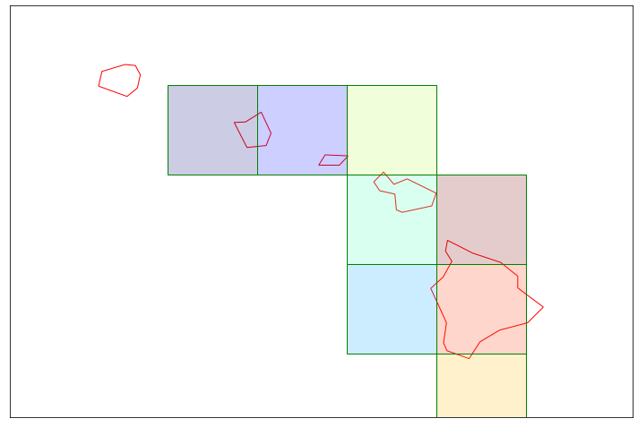
Note that polygons, which are outside of the given collection of bounding boxes, will not affect the tiling.
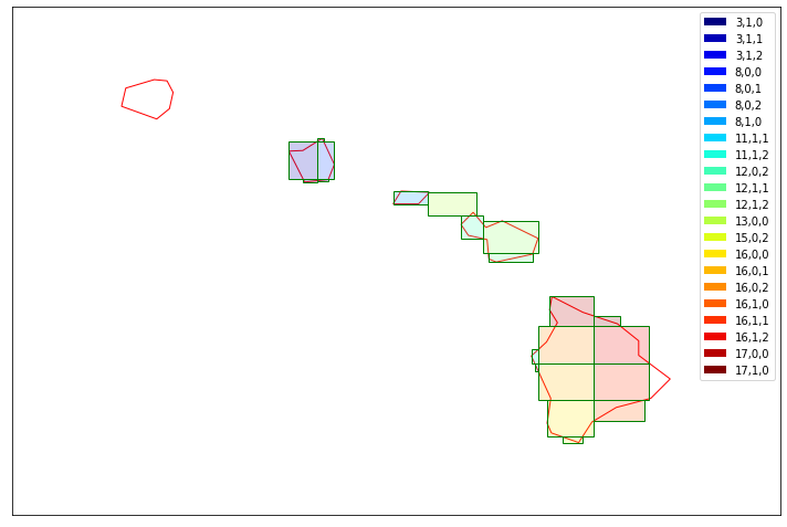
Just like in previous examples we can further split each of the bounding boxes and reduce their size to better fit given shapes.
[22]:
finer_custom_grid_splitter = CustomGridSplitter(
    [hawaii_area], CRS.WGS84, bbox_grid, bbox_split_shape=(2, 3), reduce_bbox_sizes=True
)

show_splitter(finer_custom_grid_splitter, show_legend=True)
Splitting into UTM grid zones
When dealing with large areas such as countries or continents spanning multiple UTM zones, it might be convenient to split the area according to UTM zones or to the UTM Military Grid Reference System. For these use-cases, a UtmZoneSplitter and a UtmGridSplitter have been created. These splitters will generate a list of bounding boxes in UTM CRS. Each BBox will have the CRS corresponding to the UTM zone it belongs to.
To ensure consistency across zones and grid tiles, the size of the BBoxes in metres is specified as input parameter. For this reason, the option reduce_bbox_sizes is not available for these splitters. The two splitters return consistent results between each other, with the exceptions of areas where the UTM grid tiles present exceptions, as in 31V and 32V, and 31X, 33X, 35X and 37X.
[23]:
utm_zone_splitter = UtmZoneSplitter([hawaii_area], CRS.WGS84, (50000, 50000))

show_splitter(utm_zone_splitter, show_legend=True)
[24]:
utm_zone_splitter.get_bbox_list()
[24]:
[BBox(((400000.0, 2400000.0), (450000.0, 2450000.0)), crs=CRS('32604')),
 BBox(((400000.0, 2450000.0), (450000.0, 2500000.0)), crs=CRS('32604')),
 BBox(((450000.0, 2400000.0), (500000.0, 2450000.0)), crs=CRS('32604')),
 BBox(((450000.0, 2450000.0), (500000.0, 2500000.0)), crs=CRS('32604')),
 BBox(((550000.0, 2350000.0), (600000.0, 2400000.0)), crs=CRS('32604')),
 BBox(((600000.0, 2350000.0), (650000.0, 2400000.0)), crs=CRS('32604')),
 BBox(((650000.0, 2300000.0), (700000.0, 2350000.0)), crs=CRS('32604')),
 BBox(((700000.0, 2300000.0), (750000.0, 2350000.0)), crs=CRS('32604')),
 BBox(((750000.0, 2250000.0), (800000.0, 2300000.0)), crs=CRS('32604')),
 BBox(((750000.0, 2300000.0), (800000.0, 2350000.0)), crs=CRS('32604')),
 BBox(((800000.0, 2150000.0), (850000.0, 2200000.0)), crs=CRS('32604')),
 BBox(((800000.0, 2250000.0), (850000.0, 2300000.0)), crs=CRS('32604')),
 BBox(((800000.0, 2300000.0), (850000.0, 2350000.0)), crs=CRS('32604')),
 BBox(((150000.0, 2100000.0), (200000.0, 2150000.0)), crs=CRS('32605')),
 BBox(((150000.0, 2150000.0), (200000.0, 2200000.0)), crs=CRS('32605')),
 BBox(((150000.0, 2200000.0), (200000.0, 2250000.0)), crs=CRS('32605')),
 BBox(((200000.0, 2050000.0), (250000.0, 2100000.0)), crs=CRS('32605')),
 BBox(((200000.0, 2100000.0), (250000.0, 2150000.0)), crs=CRS('32605')),
 BBox(((200000.0, 2150000.0), (250000.0, 2200000.0)), crs=CRS('32605')),
 BBox(((200000.0, 2200000.0), (250000.0, 2250000.0)), crs=CRS('32605')),
 BBox(((250000.0, 2100000.0), (300000.0, 2150000.0)), crs=CRS('32605')),
 BBox(((250000.0, 2150000.0), (300000.0, 2200000.0)), crs=CRS('32605')),
 BBox(((250000.0, 2200000.0), (300000.0, 2250000.0)), crs=CRS('32605')),
 BBox(((300000.0, 2100000.0), (350000.0, 2150000.0)), crs=CRS('32605')),
 BBox(((300000.0, 2150000.0), (350000.0, 2200000.0)), crs=CRS('32605'))]
[25]:
utm_grid_splitter = UtmGridSplitter([hawaii_area], CRS.WGS84, (50000, 50000))

show_splitter(utm_grid_splitter, show_legend=True)
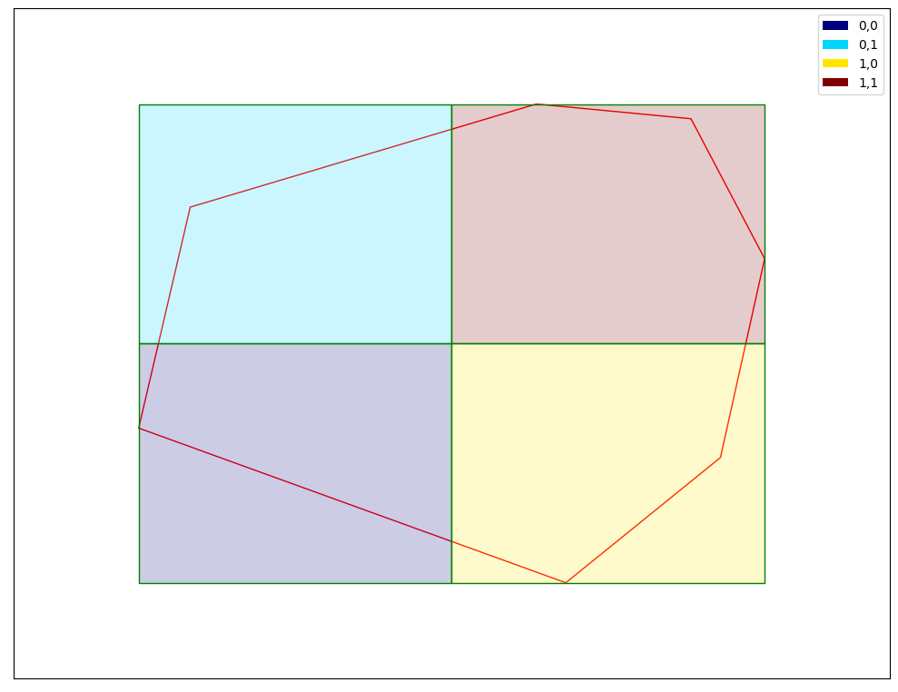
Download data from the bounding boxes using sentinelhub-py
As we can see, with the large area utilities we can easily create the bounding boxes around the desired areas. Next we are going to get the data for Kauai island (upper left), that is composed by 4 bounding boxes, to show how we can combine these utilities with the multithreaded download tools.
[26]:
kauai = hawaii_area.geoms[-1]
kauai_split = BBoxSplitter([kauai], CRS.WGS84, (2, 2))
show_splitter(kauai_split, show_legend=True)
We will use an NDVI evalscript to get example data.
[27]:
ndvi_eval = """
//VERSION=3

function evaluatePixel(samples) {
    let val = index(samples.B08, samples.B04);
    return [val];
}

function setup() {
  return {
    input: [{
      bands: [
        "B04",
        "B08",
        "dataMask"
      ]
    }],
    output: {
      bands: 1
    }
  }
}
"""
This is a helper function which returns a SentinelHubRequest for a specified bounding box. This is then applied to all bounding boxes, thus returning a list of SentinelHubRequests each with a different specified bounding box.
We save the requested TIFF files in a temporary folder, but it can be specified to another location in case it is needed.
[28]:
def get_subarea(bbox):
    return SentinelHubRequest(
        evalscript=ndvi_eval,
        input_data=[
            SentinelHubRequest.input_data(
                data_collection=DataCollection.SENTINEL2_L2A,
                time_interval=("2020-10-01", "2022-10-13"),
                mosaicking_order=MosaickingOrder.LEAST_CC,
            )
        ],
        responses=[SentinelHubRequest.output_response("default", MimeType.TIFF)],
        bbox=bbox,
        size=(1250, 1250),
        data_folder=tempfile.gettempdir(),
        config=config,
    )
[29]:
# create a list of requests
bbox_list = kauai_split.get_bbox_list()
sh_requests = [get_subarea(bbox) for bbox in bbox_list]
dl_requests = [request.download_list[0] for request in sh_requests]

# download data with multiple threads
downloaded_data = SentinelHubDownloadClient(config=config).download(dl_requests, max_threads=5)
Once the data is downloaded, we retreive all paths to the downloaded tiles.
[30]:
data_folder = sh_requests[0].data_folder
tiffs = [Path(data_folder) / req.get_filename_list()[0] for req in sh_requests]
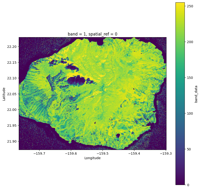
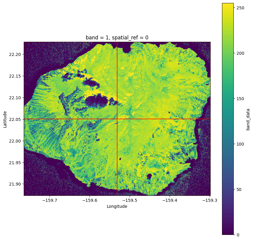
Then opening all tiles with rioxarray we mosaic the full image and plot it. Be aware though that plotting might query a lot of data if there are many large tiles. This can be very slow and consume a lot of resources.
An alternative would be to combine the tiles using the GDAL command line function gdalbuildvrt and optionally building overviews using gdaladdo so that the data can be displayed quicker at different scales.
[42]:
def plot_xr_and_bboxes(data_array, geo_vector=None):
    fig, ax = plt.subplots(figsize=(10, 10))
    data_array.plot(ax=ax)
    ax.set_ylabel("Latitude")
    ax.set_xlabel("Longitude")
    ax.set_aspect(1)
    if geo_vector is not None:
        geo_vector.plot(ax=ax, edgecolor="red", facecolor="none")
    plt.show()
[43]:
composed_tiff = xr.open_mfdataset(tiffs, engine="rasterio")
composed_map = composed_tiff.band_data.isel(band=0)

plot_xr_and_bboxes(composed_map)
Finally to visualize the bounding boxes as well we can draw the original bounding boxes over our raster.
[44]:
kauai_gpd = gpd.GeoDataFrame(geometry=[box(*bbox) for bbox in bbox_list], crs=4326)
plot_xr_and_bboxes(composed_tiff.band_data, kauai_gpd)
These separate tiles can be used well in further analysis with the eo-learn package. They can for example be ingested using the ImportFromTiffTask.
eo-learn is well suited to manage large scale and complex earth observation workflows. It does this by splitting up tasks into smaller chunks which makes large scale analysis available even with restricted resources.